Methodology
We decided to run three models: ResNet50, Xception, and YOLOv5. We ran ResNet50 and Xception models using Keras and YOLOv5 using Pytorch. We chose Keras to run ResNet50 and Xception because Keras has an application called ImageDataGenerator and its method flow_from_directory that allows us to easily augment images and keep the file structure given by the original authors. All of our code was run using Google Colab Pro. For ResNet50 and Xception we did an 80%, 10%, 10% split on the data, and for YOLOv5 we did a 90%, 10% split, leaving at least four images in each cell class type.
Image Augmentation for Keras Models:
While we varied several preprocessing tasks and hyperparameters in our training of many different versions of the ResNet50 and Xception models, our final and best performing iterations of both models includes the following; like the previous paper’s implementation, we created augmented images by randomly rotating the images somewhere between 0 and 359 degrees and horizontally or vertically flipping the image. These methods were inspired by those used by Matek et al. We filled in blank spots on the transformed images by filling them in with reflections of the original image. Unlike Matek et al.’s paper, however, we took a different overall approach to this in order to assuage some of the suspicions we had about leakage as well as our skepticism about equalizing very radically imbalanced classes through augmentation to the same number of images (close to the number of images in the larger classes - 10,000). Instead, each epoch during training augmented the images differently in a random fashion. This was done through use of the keras.preprocessing.image ImageDataGenerator function which also allows for preprocessing and augmentation during training instead of saving augmented images and then training each model from those saved images.
While we varied several preprocessing tasks and hyperparameters in our training of many different versions of the ResNet50 and Xception models, our final and best performing iterations of both models includes the following; like the previous paper’s implementation, we created augmented images by randomly rotating the images somewhere between 0 and 359 degrees and horizontally or vertically flipping the image. These methods were inspired by those used by Matek et al. We filled in blank spots on the transformed images by filling them in with reflections of the original image. Unlike Matek et al.’s paper, however, we took a different overall approach to this in order to assuage some of the suspicions we had about leakage as well as our skepticism about equalizing very radically imbalanced classes through augmentation to the same number of images (close to the number of images in the larger classes - 10,000). Instead, each epoch during training augmented the images differently in a random fashion. This was done through use of the keras.preprocessing.image ImageDataGenerator function which also allows for preprocessing and augmentation during training instead of saving augmented images and then training each model from those saved images.
ResNet50
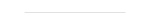
We decided to use ResNet50 as it is the precedent of ResNext, the model Matek et al. used, which is known to perform well on image classification tasks. We augmented the images as specified above, and also rescaled the images by 1/255. While training ResNet, we decided to run certain implementations utilizing data augmentation and not utilizing data augmentation as a baseline. A full breakdown of the ResNet models we ran and reasoning for running these models can be found below.
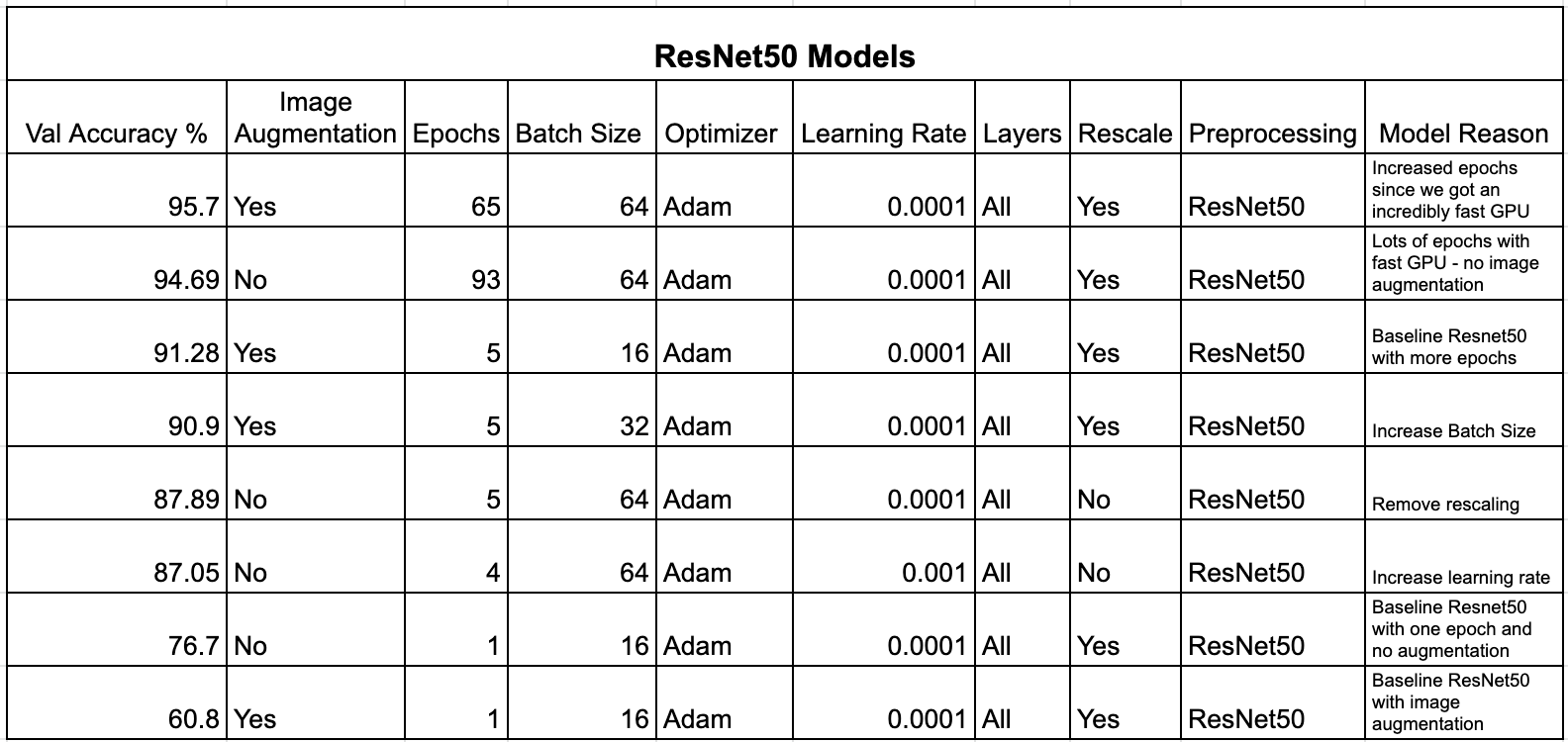
The ResNet model with the highest accuracy on the validation set yielded an accuracy of 95.7%. The model included the image augmentation mentioned above and was run for 65 epochs with a batch size of 64 using Adam optimizer with a learning rate of 0.0001. This model yielded an accuracy of 95.51% on the test set. Below is a confusion matrix of the test results.
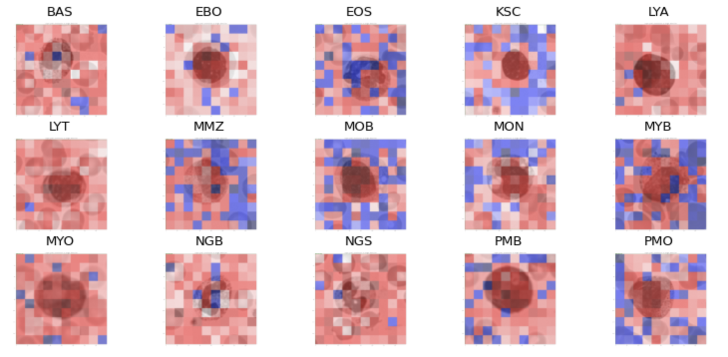
As can be seen from the confusion matrix, the model performed the best on NGS, MYO, MON, LYT, and EOS which is to be expected since these are the cell classes with the most images. This accuracy is quite high so we decided to look at a heatmap to determine what the model was looking at to create these predictions.
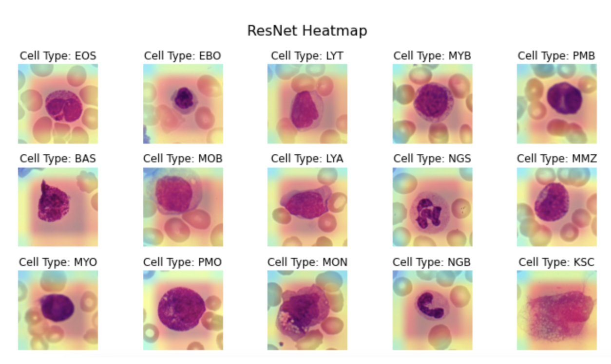
As can be seen from the heatmap, the model focuses on a square-like shape around the cell meaning the model is using the cell to make the prediction and not the surrounding cells or other features we did not take into consideration.
Xception
The Xception model was a logical next step in order to improve results over the ResNet50 model. In several benchmarks for similar multiclass image classification models, the Xception model performed better than the ResNet50 model and remains of reasonable size and depth to be able to train on Google Colab (Chollet et al., 2015). Furthermore, the Xception model is predefined in Keras and can follow a similar notebook structure to the ResNet50 model, allowing for ease of implementation and comparison. We augmented the images similarly to the ResNet50, other than skipping the overt rescaling to 1/255. Like the ResNet50 model, we ran models with and without image augmentation to achieve the best performing model, eventually selecting a model with image augmentation. We also varied learning rate, batch size, and number of epochs. A full breakdown of the Xception models we ran and reasoning for running these models can be found below.
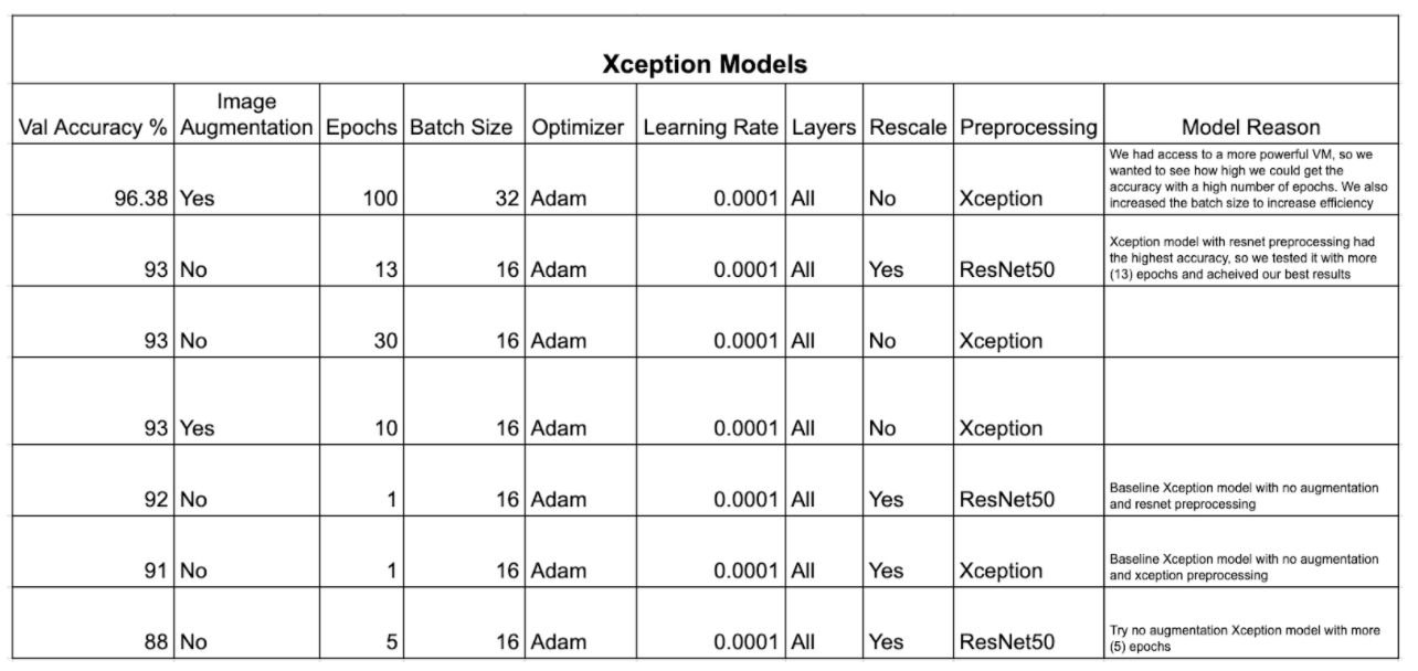
The Xception model with the highest accuracy on the validation set yielded an overall accuracy of 96.38%. The model included the image augmentation mentioned above and was run for 100 epochs with a batch size of 32 using Adam optimizer with a learning rate of 0.0001. The best accuracy was achieved at the 39th epoch, so weights for the final model were loaded from the 39th epoch weight checkpoint of this model. This model yielded an overall accuracy of 96.05% on the test set. Below is a confusion matrix of the test results.
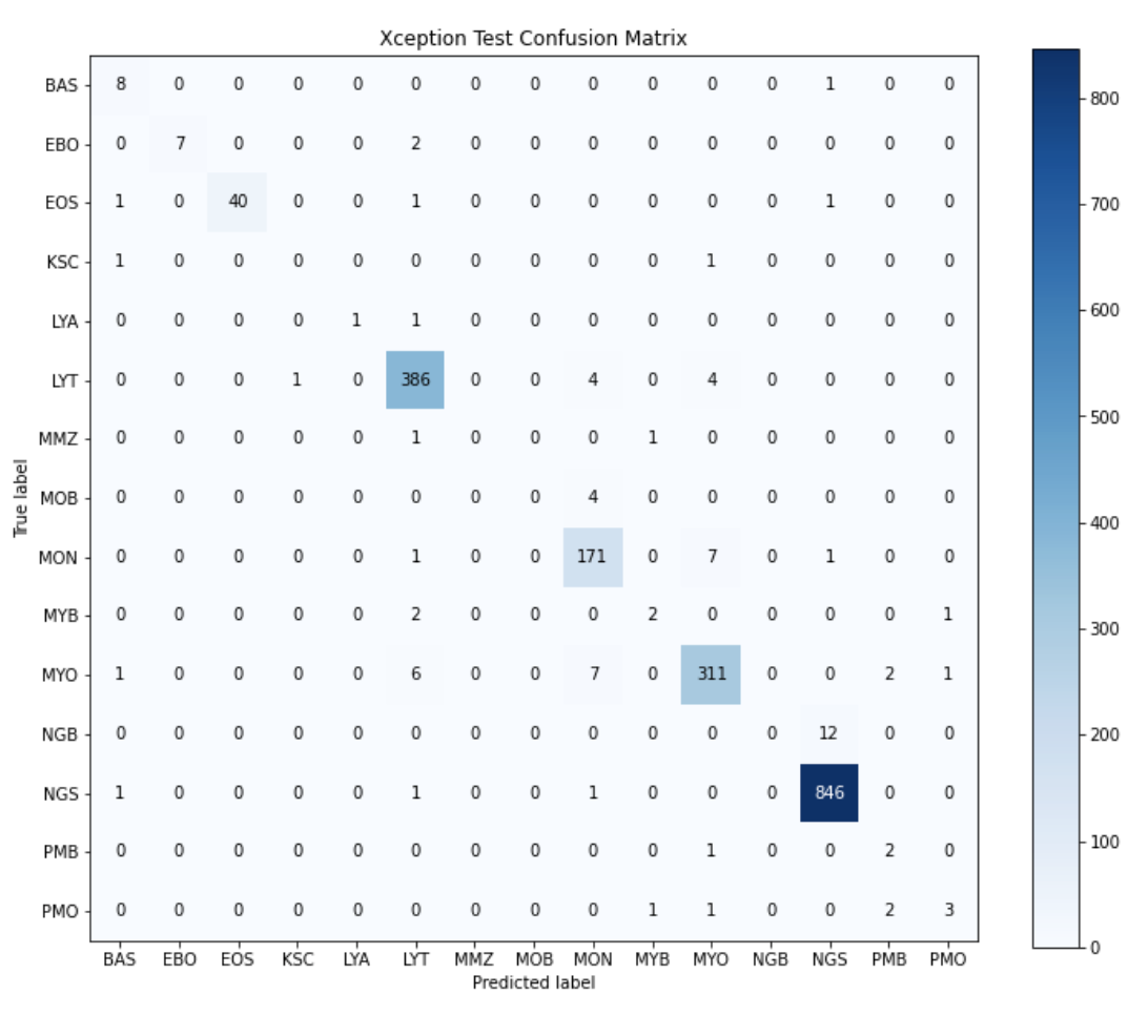
As can be seen from the confusion matrix, like the ResNet50 model, this model performed the best on NGS, MYO, MON, LYT, and EOS which is to be expected since these are the cell classes with the most images. This accuracy is quite high so we decided to look at a heatmap to determine what the model was looking at to create these predictions.
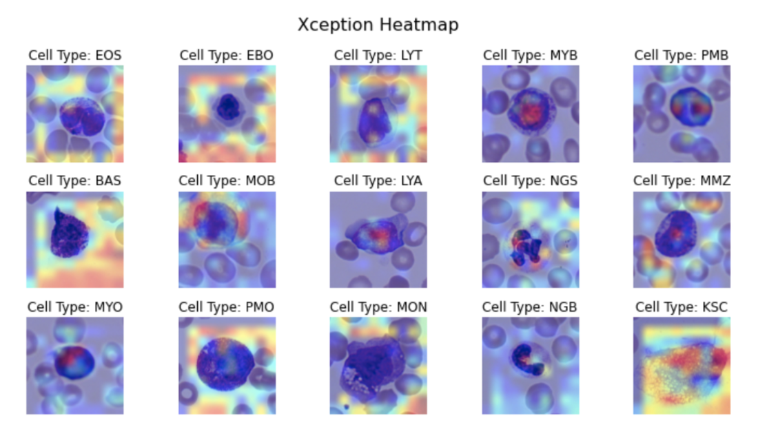
As seen above, the Xception heatmaps appear very different from the ResNet50 heatmaps. Important pixels are much more specific to areas of the cells rather than showing a general area of red around the cell. In the PMB heatmap, which is a bilobed cell type, it can even be seen that the model recognizes the two different lobes. The focus on points within the cell also, like with the ResNet50 model, helps to rule out leakage or other suspicious behavior by the model.
YOLOv5
YOLOv5 is a power object detection model pre-trained on the COCO dataset that is often used for real time object detection. There are four versions of YOLOv5 that vary in size; we chose to use the smallest version which has 7.3 million parameters (while the largest has 87.7 million). One of the advantages of YOLOv5 is that it can be trained to detect multiple objects in a single image. Thus, the model could provide a means for us to be able to do white blood cell identification in multicell images. Another strength of YOLOv5 is its ability to learn objects with relatively low sets of training images; this helped address some of the class imbalances in the training data.
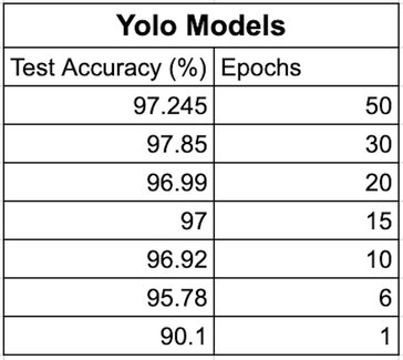
We started training our model with 1 epoch and increased to 6, 10, 15, 20, 30, and 50 epochs. The highest overall test accuracy is 97.85% at 30 epochs.
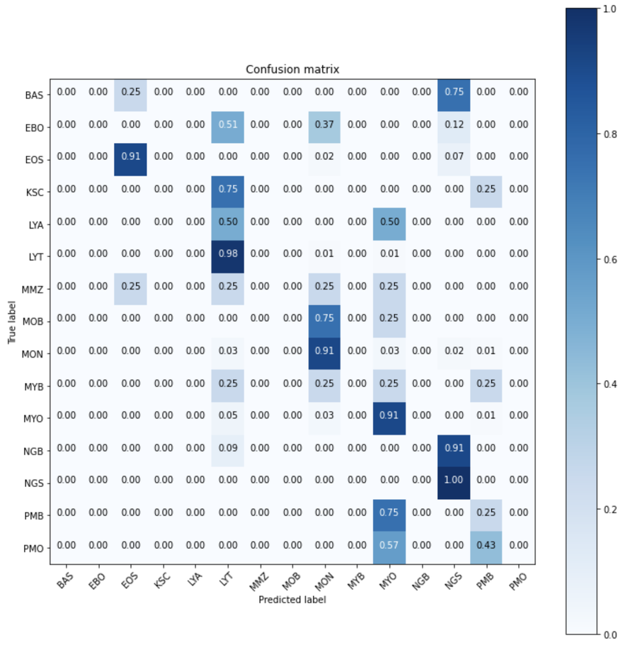
From the confusion matrix, the model performed the best on EOS, LYT, MON, MYO, and NGS. This is expected because these white blood cell types all have a large number of images in the training set.
The 15 heatmaps below show what areas of the single cell images the model focussed on to make its classification for one example per class. Darker red corresponds to more focus and darker blue areas correspond to less focus. We see that in general the model is focussing on the majority of the image with a trend toward the center of the image, which is the cell of interest.